Optimising Last-Mile Delivery using Open Source

Last-mile delivery can become tedious if not planned in order. This blog will explain how we can use ORS API openrouteservice.org and K-Means clustering techniques in python to segregate the delivery locations and generate trip sheets for each despatch.
Delivery is dependent on various parameters. Based on my recent work for a company, I have documented the workflow I used to solve their last-mile delivery challenge.
Problem statement
Daily delivery volume ~300 locations.
The company has eight vehicles, and each vehicle can carry only ~15-18 delivery items in a single trip.
After the final trip for a vehicle, it may/may-not return to the warehouse.
Input
An excel sheet containing 300 addresses.
Workflow
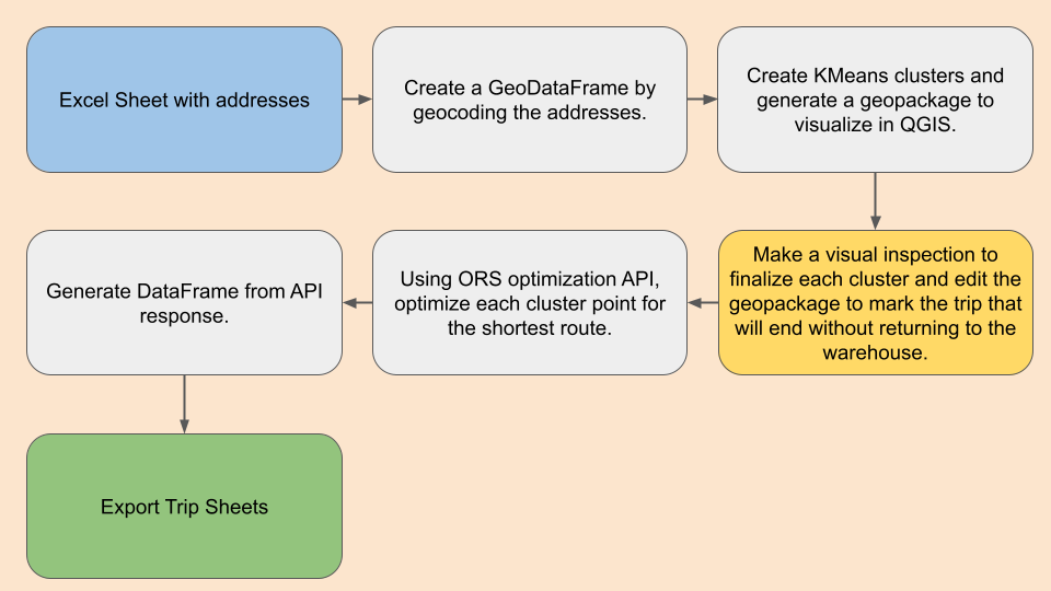
Geocoding
Nominatim can be used to geocode addresses, and this uses OpenStreetMap data for geocoding. For addresses in a few hundred, the API version can be used, and for power users, follow this link to learn more about deploying this database at your premises.
A demo for getting the address for a few public parks in Chennai is shown here.
# Park Names

# Originally this is giving in excel file with 300 delivery location.
# To know about excel import in python see
# https://pandas.pydata.org/docs/reference/api/pandas.read_excel.html

parks = ['Anna Tower, Chennai',
         'Natesan Park, Chennai',
         'Arignar Anna Park',
         'Semmozhi Poonga, Chennai']

# Get address and coordinate information.
geolocator = Nominatim(user_agent="key")
loc = {'Name':[], "Address":[], "Latitude":[], "Longitude":[]}
for park in parks:
    address = geolocator.geocode(park)
    coordinate = (address.latitude, address.longitude)
    loc['Name'].append(park)
    loc['Address'].append(address)
    loc['Latitude'].append(coordinate[0])
    loc['Longitude'].append(coordinate[1])
    time.sleep(1)
Create a GeoDataFrame, pass the Latitude and Longitude information to generate point geometry for each address.
# Generate a GeoDataframe
df = geopandas.GeoDataFrame(loc, columns=loc.keys(),
                          geometry=geopandas.points_from_xy(loc['Longitude'], loc['Latitude']))
print(df)
output
| index | Name | Address | Latitude | Longitude | geometry |
| 0 | Anna Tower, Chennai | Anna Nagar Tower Park, CMWSSB Division 100, Ward 100, Zone 8 Anna Nagar, Chennai, Chennai District, Tamil Nadu, 600001, India | 13.08705145 | 80.2142726498145 | POINT (80.2142726498145 13.08705145) |
| 1 | Natesan Park, Chennai | Natesan Park, CMWSSB Division 136, Ward 136, Zone 10 Kodambakkam, Chennai, Chennai District, Tamil Nadu, 600001, India | 13.0375196 | 80.23640685816439 | POINT (80.23640685816439 13.0375196) |
| 2 | Arignar Anna Park | Arignar Anna Zoo Park, Grand Southern Trunk Road, Peerkankaranai, Irumbuliyur, Tambaram, Chengalpattu, Chengalpattu District, Tamil Nadu, 600045, India | 12.8835357 | 80.09161214679824 | POINT (80.09161214679824 12.8835357) |
| 3 | Semmozhi Poonga, Chennai | செம்மொழி பூங்கா, Cathedral Road, CMWSSB Division 118, Ward 118, Zone 9 Teynampet, Chennai, Chennai District, Tamil Nadu, 600001, India | 13.0506255 | 80.2515099 | POINT (80.2515099 13.0506255) |
Notice the last column, its contains data of type shapely geometry. The geometry column can be used to represent this data as a spatial layer.
Clustering
Once the addresses are plotted as geographic coordinates, we can use machine learning algorithms to segregate them into small groups. For this process, I used a popular grouping technique KMeans clustering. In this algorithm number of clusters can be defined, and the algorithm will fix centroids and group the points. To understand the working of this algorithm I encourage to read this blog K-means Clustering: Algorithm, Applications, Evaluation Methods, and Drawbacks.
Illustration showing diffrent centroids during clustering process(image from wikipedia)
But here the catch is each cluster may/may not have an equal number of points. So I used the Constrained K-Means Clustering technique, where we can specify cluster's minimum and maximum size. This is implemented using the library k-means-constrained
With the minimum value set to 15 and the maximum set to 18, we can group the 300 locations into ~20 groups.
# Setting the cluster minimum and maximum size
min_size = 15
max_size = 18

# Finding the total delivery points, clustering algorithm accept only X and Y value in numpy format
# Hence extracting the latitude and longitude information and converting the DataFrame as numpy.
latlon = df[['Longitude', 'Latitude']].to_numpy()
total = latlon.shape[0]

# Finding the maximum total cluster.
total_clusters = int(total/max_size) + 1

clusters = KMeansConstrained(n_clusters=total_clusters,
                               size_min=min_size,
                               size_max=max_size,
                              random_state=0)
clusters_values  = clusters.fit_predict(latlon)
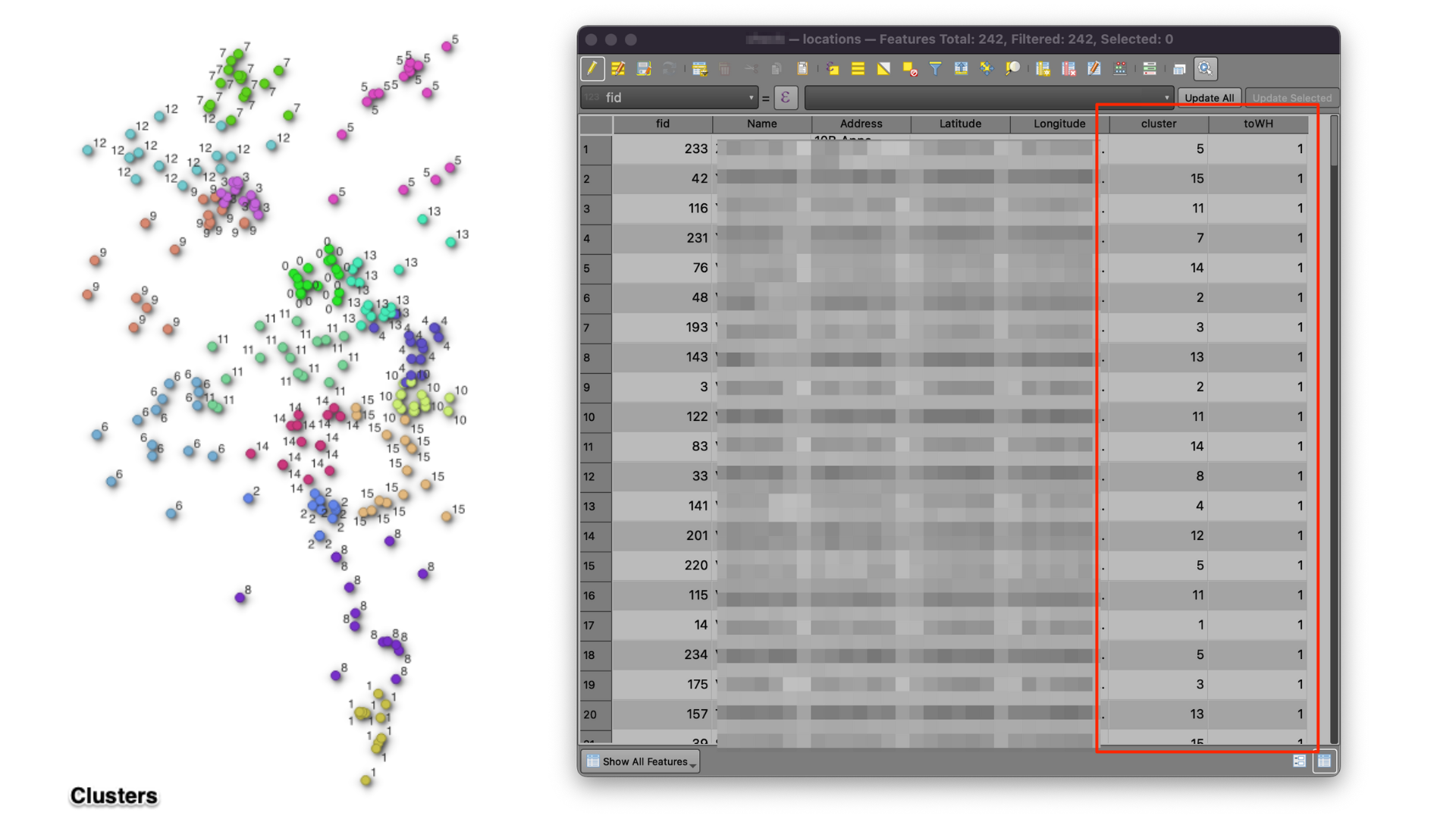
Once the clusters are generated, the data is cast as GeoDataFrame using GeoPandas. Then a geopackage output is generated. As we know, no clustering algorithm can generate clusters as expected by humans, and also, the cluster size will vary depending upon other factors like vehicle capacity, etc. Hence using the geopackage despatcher can conveniently modify cluster groups in QGIS. This also helps to input the return condition for the cluster.
# write cluster numbers to GeoDataFrame

df['cluster'] = clusters_values

# Create a new column return and set it to true 1.
# Dispatcher can modify this based on his needs.

df['toWH'] = 1

# Create GeoDataFrame
gdf = geopandas.GeoDataFrame(df, geometry=geopandas.points_from_xy(df.Longitude, df.Latitude))


# Write the GeoDataFrame as GeoPackage.
folder = 'demo'
file = 'clusters.gpkg'
path_gpkg = os.path.join(date, folder)
gdf.to_file(path_gpkg, layer='locations', driver="GPKG")
Checking and Modifying the data.
QGIS is an open-source geospatial software. It is easy to visualize spatial layer and find the underlying pattern. Also QGIS editing capability will be very helpfull for minor updations.
Load the GeoPackage into the canvas. Using the layer styling panel in QGIS, each cluster is styled in a different colour. The OpenStreetMap base map can be loaded for the road network, and a visual inspection is done for each cluster. If any point needs modification using the Attribute table's edit feature, the cluster groups can be changed. Also, by default, the back to the warehouse (reverse) is true for all clusters. Dispatcher can also modify this based on the driver's availability and cluster location.
To know more about editing in the attribute table, read QGIS documentation..
Once all the changes are done, the GeoPackage is saved.
Optimize clusters
A function is created to take location and generate an optimized delivery route. While passing the delivery location, we can pass the condition for return status for the cluster.
#warehouse
wh = [lon,lat]
def route_optimize(cluster):
vehicles = []
deliveries = []
cluster_df = df[df['cluster']==cluster]
return_condition = list(cluster_df['toWH'])[0]
for delivery in cluster_df.itertuples():
deliveries.append(ors.optimization.Job(id=delivery.Index, location=[delivery.Longitude, delivery.Latitude]))
# Set vechile condition based on the return condition
if return_condition:
vehicles.append(ors.optimization.Vehicle(id=0,start=list(wh), end=list(wh)))
else:
vehicles.append(ors.optimization.Vehicle(id=0,start=list(wh)))
ors_client = ors.Client(key=passcode)
result = ors_client.optimization(jobs=deliveries, vehicles=vehicles, geometry=True)
li = result['routes'][0]['steps']
li2 = []
for n, x in enumerate(li):
lon = x['location'][0]
lat = x['location'][1]
li2.append([n, lat, lon])
order_df = pd.DataFrame(li2, columns=['order', 'lon', 'lat'])
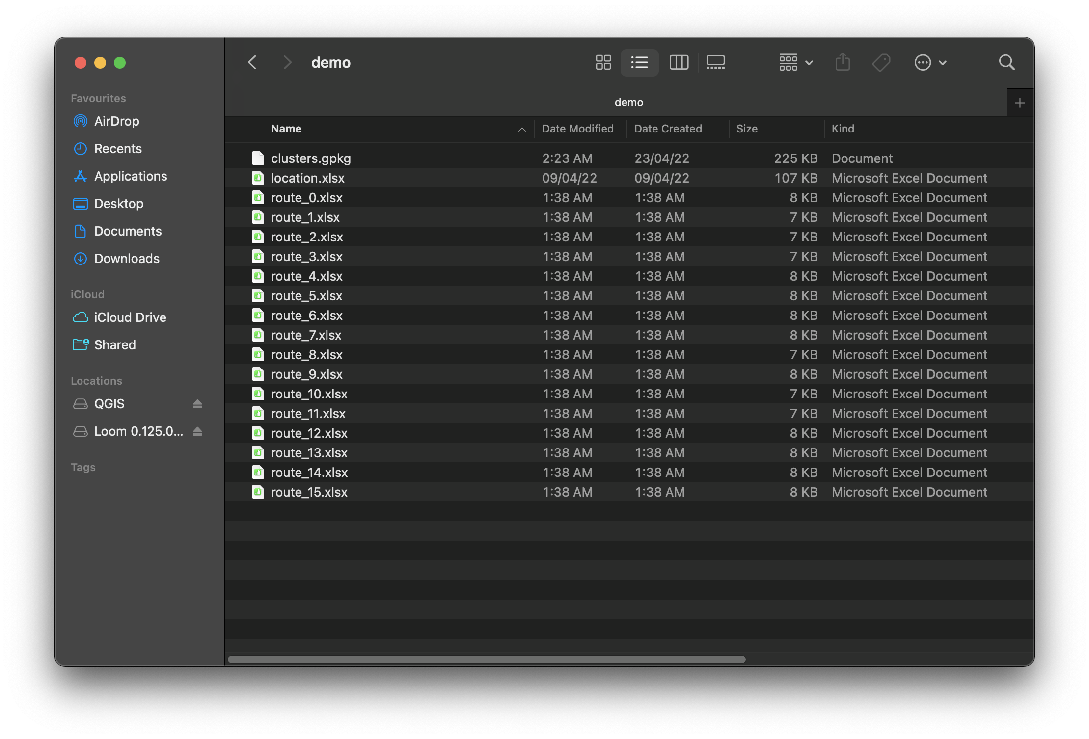
file_name = 'route_' + str(int(return_condition)) + '.xlsx'
path_excel = os.path.join(folder, file_name)
order_df.to_excel(path_excel)
return path_excel
The below graphics will show how return optimization is vital for delivery planning.

To optimize each cluster, each cluster number is passed on to the function, and the DataFrame is filterer for that cluster. Once the specified group is obtained using the latitude and longitude location information obtained for constructing the API call. Then based on the return condition for the cluster vehicles, conditions are set.
Using these parameters, an API request to Open Route Service optimization API service is made. Finally, we can generate a DataFrame and convert it into a despatch file in excel format using the response received.
df = geopandas.read_file(path_gpkg, layer='locations')

#Get total clusters
total_cluster =  list(df['cluster'].unique())

for n in total_cluster:
    print(route_optimize(n), ' file written successfully')
Conclusion.
This workflow is based on Open Data, and the live traffic is not available for route planning. The fastest route is chosen based on each road speed limit available on the open street map. This can be a downside, but this workflow has made daily planning easy and saves huge time, money, and human resources for the company in the dispatching process.
Disclaimer : The data I used is the property of the company, hence it cannot be shared publicly. All the map shown here are generate with randomised value with the data.
To access the notebook visit : GitHub


